RNN을 사용해 감성분석을 진행하는 경우는 Many-to-One Model을 사용하는 경우
LSTM 은 장기기억이 가능하기 때문에 부정적인 단어가 소멸되는 것을 막을 수 있음
두 개의 실습 진행
1) IMDB 테스트코드
- tensorflow tfds dataset의 imdb_reviews (약 25000개의 학습/테스트 데이터셋)
- string 형태의 데이터 사용
- 레이블 : 긍정,부정 으로 이진분류모델
2) 네이버 테스트코드
- 15만개의 학습 5만개 테스트 데이터셋
- 레이블 : 긍정,부정으로 이진분류모델
=> 언어에 대한 처리방법은 영어든 한국어든 기본적으로는 동일하나, 한국어는 토큰화를 진행할 때 형태소 분석기를 사용한다는 차이점이 있음. 전처리 방법에서 한글 이외의 것은 삭제하거나 불용어 처리해주어야함. 띄어쓰기 때문에 한글 형태소 분석기도 필요
//형태소 분석기 사용
from konlpy.tag import Okt
	okt = Okt()
    okt.morphs("아버지가방에들어가신다")
    ['아버지','가방','에','들어가신다']
IMDB 테스트코드
필요한 라이브러리 임포트 진행
import tensorflow as tf
from tensorflow.keras.layers import Dense, LSTM, Embedding, Dropout, Bidirectional
from tensorflow.keras.models import Sequential
from tensorflow.keras.preprocessing.text import Tokenizer
from tensorflow.keras.preprocessing.sequence import pad_sequences
import tensorflow_datasets as tfds
import numpy as np
import matplotlib.pyplot as plt
데이터셋과 정보 가져오기 (25000개씩 확인 가능)
dataset, info = tfds.load('imdb_reviews', with_info=True, as_supervised=True)
train_dataset, test_dataset = dataset['train'], dataset['test']
len(train_dataset), len(test_dataset)
데이터 읽어보기 (텐서형태이기 때문에 for문으로 확인해야함..한개만 확인해보기)
for input, label in dataset['test']:
	print(label)
	print(input)
	break
전처리 진행
train_sentences = []
train_labels = []
test_sentences = []
test_labels = []

for sent, label in train_dataset:
	train_sentences.append(str(sent.numpy()))
	train_labels.append(label.numpy())

for sent, label in test_dataset:
	test_sentences.append(str(sent.numpy()))
	test_labels.append(label.numpy())

print(train_labels[-1])
print(train_sentences[-1])

print(test_labels[-1])
print(test_sentences[-1])
데이터를 학습에 필요한 넘파이로 변경 후 진행
train_labels = np.array(train_labels)
test_labels = np.array(test_labels)

print(train_labels.shape)
print(test_labels.shape)
토큰화 진행
vocab_size = 10000
tokenizer = Tokenizer(num_words = vocab_size, oov_token='<OOV>')
tokenizer.fit_on_texts(train_sentences)
훈련이 잘 됐나 확인
#각 10000개씩 만들어졌나 확인
tokenizer.index_word
tokenizer.word_index
데이터를 수열(sequence)로 변환
train_sequences = tokenizer.texts_to_sequences(train_sentences)
test_sequences = tokenizer.texts_to_sequences(test_sentences)

#첫번째거 확인해보기
print(train_sequences[0])
print(test_sequences[0])
히스토그램으로 데이터 빈도수 분포 확인
plt.hist([len(s) for s in train_sequences] + [len(s) for s in test_sequences]))
plt.show()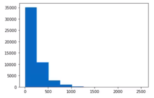
간격이 너무 넓으니 bins 조정을 주어서 촘촘하게 다시 그려보면
#파이썬 문법중 리스트 컴프리헨션 활용
plt.hist([len(s) for s in train_sequences] + [len(s) for s in test_sequences]), bins=50)
plt.show()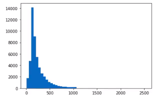
요렇게 확인해볼수 있다.
필요한만큼 데이터 잘라서 패딩 진행
max_length = 150
'''
'pre'는 앞쪽에 채우는거, 'post'는 뒤쪽에 채우는거 감성분석은 대개 앞쪽에 데이터가 중요해서
post로 뒤쪽에 채우고, 번역같은 경우는 pre로 채우는경우도 많음
'''
train_padded = pad_sequences(train_sequences,maxlen=max_length, truncating='post', padding='post')
test_padded = pad_sequences(test_sequences,maxlen=max_length, truncating='post', padding='post')

print(train_padded.shape)
print(test_padded.shape)
print(train_padded[0])
print(test_padded[0])
수열로 된 데이터를 다시 reverse 해서 확인해보기
reverse_word_index = dict([(value, key) for (key, value) in tokenizer.word_index_items()])

def decode_review(sequence):
	#리스트 컴프리헨션
	return ' '.join([tokenizer.index_word.get(i, '<pad>') for i in sequen

print(decode_review(train_padded[0]))
print(train_sentences[0])
데이터 준비가 완료됐으니 모델을 만들기
#방법 1
model = Sequential()
model.add(Embedding(vocab_size+1 , 64)) # +1 은 pad해줬으니까
model.add(Bidirectional(LSTM(64)))
model.add(Dense(64, activation='relu'))
model.add(Dense(1, activation='sigmoid'))
model.summary()

#방법 2
model = Sequential([
	Embedding(vocab_size+1, 64),
	Bidirectional(tf.keras.layers.LSTM(64)),
	Dense(64, activation='relu'),
	Dense(1, activation='sigmoid')
])
model.compile(loss='binary_crossentropy',optimizer='adam', metrics=['accuracy'])
model.summary()
모델학습진행
num_epochs = 30
history = model.fit(train_padded, train_labels, epochs=num_epochs, batch_size=128,
			validation_data=(test_padded, test_labels), verbose=1)
oop 형식의 그래프로 확인
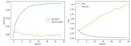
fig, (ax1, ax2) = plt.subplots(1,2,figsize=(12,4))

ax1.plot(history.history['accuracy'], label='accuracy')
ax1.plot(history.history['val_accuracy'], label='val_accuracy')
ax1.set_xlabel('Epochs')
ax1.set_ylabel('accuracy')
ax1.legend(['accuracy','val_accuracy'])

ax1.plot(history.history['loss'], label='loss')
ax1.plot(history.history['val_loss'], label='val_loss')
ax1.set_xlabel('Epochs')
ax1.set_ylabel('loss')
ax1.legend(['loss','val_loss'])
plt.show()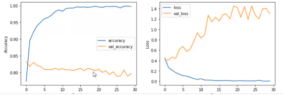
데이터가 25000개뿐이라 결과가 몹시 안좋게 나왔다... 열배는 더 있어야하지만 테스트해본거에 의의를 두어야할듯..
이미지 데이터 모델같은 경우는 25000개도 괜찮겠지만 언어모델은 몇십만개는 있어야하는데 GPU 성능도 있어야하구 여러가지 제약이 더 많은듯..
이후 모델 활용해보기
sample_text = ['The Movel was terrible, I would not recommend the movie']

#모델과 마찬가지로 수열변환, 패딩진행
sample_seq = tokenizer.texts_to_sequences(sample_text)
sample_padded = pad_sequences(sample_seq, maxien=max_length, padding='post', truncating='post')

#모델에 입력으로 주기
model.predict(sample_padded)
'''
1에 가까우면 긍정으로 판단
0에 가까우면 부정으로 판단
'''
네이버 영화감상평 테스트코드
필요한 라이브러리 설치&임포트
!pip install -q KoNLPyimport numpy as np
import pandas as pd
import re
import time
import matplotlib.pyplot as plt
from konlpy.tag import Okt
import tensorflow as tf
from tensorflow.keras.preprocessing.text import Tokenizer
from tensorflow.keras.preprocessing.sequence import pad_sequences
from tensorflow.keras.models import Sequential
from tensorflow.keras.layers import Embedding, Bidirectional, Dense, LSTM
데이터는 구글드라이브에 마운트 하거나 깃허브로 연동하거나 등등 편한 방법을 사용하면 된다
여기 글에서는 별도로 데이터는 올리진않고 네이버 영화평 데이터 검색하면 얻을 수 있다! (약 15만건)
null 제거
train_data.dropna(inplace=True)
test_data.dropna(inplace=True)
null 이 제거되었는지 확인
train_data.isnull().sum(), test_data.isnull().sum()okt.morphs() 로 형태소 분석
okt = Okt()
test = "아버지가방에들어가신다"
okt.morphs(test, stem=True)

#['아버지', '가방', '에', '들어가다']
텍스트 전처리 진행
#불용어 제거
def preprocessing(sentence, remove_stopwords=True):
    #stop_words = set(['에', '은', '는', '이', '가', '그리고', '것', '들', '수', '등', '로', '을', '를', '만', '도', '아', '의', '그', '다'])
	stop_words = []

	sentence = re.sub('\\\\n', ' ', sentence) # 개행문자 제거
	sentence = re.sub('[^가-힣ㄱ-ㅎㅏ-ㅣ ]', '', sentence) #한글외에 모두 제거
	sentence = okt.morphs(sentence, stem=True)
	if remove_stopwords:
		sentence = [token for token in sentence if not token in stop_word
	return sentence
train_sentences = []
train_labels = []
test_sentences = []
test_labels = []
start = time.time() #시간확인용
'''
IMDB하고 거의 비슷
IMDB는 데이터 input과 레이블이 같이 데이터에 있었지만 네이버는 따로 컬럼이 분리되어있어서 enumerate로
zip 페어링을 진행해줌
'''
for i, (sent, label) in enumerate(zip(train_data['document'], train_data['label'])):
if i % 10000 == 0:
print(f"Train processed = {i}")#확인용 로그 출력
sent = preprocessing(sent) #한글 외에는 전처리 된거로 받음
if len(sent) > 0:
train_sentences.append(sent)
train_labels.append(label)
for i, (sent, label) in enumerate(zip(test_data['document'], test_data['label'])):
if i % 1000 == 0:
print(f"Test processed = {i}")
sent = preprocessing(sent)
if len(sent) > 0:
test_sentences.append(sent)
test_labels.append(label)
print(time.time() - start)넘파이 배열로 변환
train_labels = np.array(train_labels)
test_labels = np.array(test_labels)

print(train_labels.shape)
print(test_labels.shape)
수열변환
VOCAB_SIZE = 20000

tokenizer = Tokenizer(num_words=VOCAB_SIZE, oov_token="<OOV>")
tokenizer.fit_on_texts(train_sentences)

train_sequences = tokenizer.texts_to_sequences(train_sentences)
test_sequences = tokenizer.texts_to_sequences(test_sentences)

print(train_sequences[0])
print(test_sequences[0])
리스트컴프리헨션을 이용해 히스토그램으로 빈도수 시각화
plt.hist([len(s) for s in train_sequences] + [len(s) for s in test_sequences], bins=30);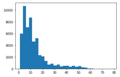
아까 IMDB에 비해 문장 길이가 짧음을 알 수 있음
다시 한글로 된 문장으로 reverse
reverse_word_index = dict([(v, k) for (k, v) in tokenizer.word_index.items()])

def decode_sentence(sequence):
	return ' '.join([reverse_word_index.get(i, '?') for i in sequence])

print(decode_sentence(train_padded[4]))
print(train_sentences[4])
모델만들기
model = Sequential([
	Embedding(VOCAB_SIZE+1, 64),
	Bidirectional(LSTM(64)),
	Dense(32, activation='relu'),
	Dense(1, activation='sigmoid')
])

model.compile(loss='binary_crossentropy', optimizer='adam', metrics=['accuracy'])
model.summary()
모델훈련
num_epochs = 30
history = model.fit(train_padded, train_labels, epochs=num_epochs, batch_size = 128,
		validation_data=(test_padded, test_labels), verbose=1)
시각화 진행
fig, (ax1, ax2) = plt.subplots(1, 2, figsize=(12, 4))

ax1.plot(history.history['accuracy'])
ax1.plot(history.history['val_accuracy'])
ax1.set_xlabel('Epochs')
ax1.set_ylabel('accuracy')
ax1.legend(['accuarcy', 'val_accuracy'])

ax2.plot(history.history['loss'])
ax2.plot(history.history['val_loss'])
ax2.set_xlabel('Epochs')
ax2.set_ylabel('loss')
ax2.legend(['loss', 'val_loss'])
plt.show()
샘플데이터 적용해보기
sample_text = ['이 영화는 정말 짜증나서 못 보겠다']

sample_seq = tokenizer.texts_to_sequences(sample_text)

sample_padded = pad_sequences(sample_seq, maxlen=max_length, padding='post
결과 보기
model.predict([sample_padded])
#0 에 가까우면 부정 1 에 가까우면 긍정
이후 임베딩 레이어에서 vects.tsv 파일과 meta.tsv 파일을 write 해주고
https://projector.tensorflow.org/ 여기 사이트를 활용해 3차원으로 시각화 해볼 수 있다. 해당 사이트 가이드라인을 참고하면 도움이 될 듯하다
out_v = open('vects.tsv', 'w', encoding='utf-8')
out_m = open('meta.tsv', 'w', encoding='utf-8')

for i in range(1, 1000):
    word = tokenizer.index_word.get(i, '?')
    embeddings = weights[i]
    out_m.write(word+'\n')
    out_v.write('\t'.join([str(x) for x in embeddings]) + '\n')

out_v.close()
out_m.close()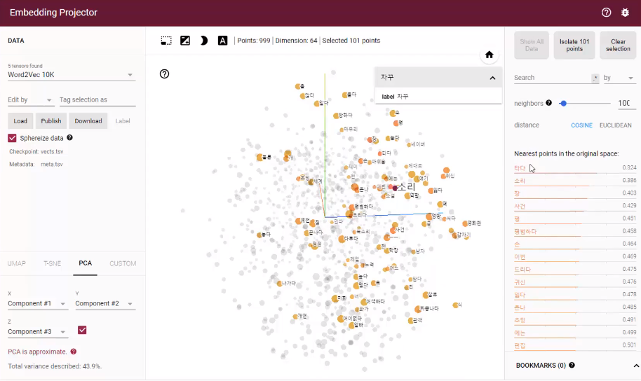
'스터디 > AI' 카테고리의 다른 글
| [Imple] yolo 모델 불량검출 (0) | 2023.04.13 |
|---|---|
| [실무] 자연어처리에 토큰화 (0) | 2023.04.10 |
| [이론] 자연어처리 RNN (0) | 2023.03.17 |
| [이론] 자연어처리 intro (2) | 2023.03.17 |
| [실무] bentoML 라이브러리 (0) | 2023.03.04 |